Introduction to Fortran

Note

To learn any new programming language good learning resources are important. This introduction covers the basic language features you will need for this course but Fortran offers much more functionality.

Good resources can be found at fortran-lang.org. Especially the learn category offers useful introductory material to Fortran programming and links to additional resources.

The fortran90.org offers a rich portfolio of Fortran learning material. For students with prior experience in other programming languages like Python the Rosetta Stone might offer a good starting point as well.

Also, the Fortran Wiki has plenty of good material on Fortran and offers a comprehensive overview over many language features and programming models.

An active forum of the Fortran community is the fortran-lang discourse. While we offer our own forum solution for this course to discuss and troubleshoot, you are more than welcome to engage with the Fortran community there as well. Just be mindful when starting threads specific to this course and tag them as Help or Homework.

General Principles

Programming is the art of telling a computer what to do, usually to perform an action or solve a problem which would be too difficult or laborious to do by hand. It thus involves the following steps:

1. Understanding the problem.

2. Formulating an approach/algorithm to the problem.

3. Translating the algorithm into a computer–compatible language: Coding

4. Compiling and running the program.

5. Analyzing the result and improving the program if necessary or desired.

This manual assumes that steps 1 and 2 have already been taken care of in the Quantum Chemistry I module. We will thus concern ourselves with the problems of translating an algorithm or a formula, spelled out on paper, to something the computer understands first.

Compiling and Running a Program

Before beginning to write computer code or to code in short, one needs to choose a programming language. Many of them exist: some are general, some are specifically designed for a task, e.g. web site design or piloting a plane, some have simple data structures, some have very special data structures like census data, some are rather new and follow very modern principles, some have a long history and thus rely on time-tested concepts.

In the case of this module, the Fortran programming language is chosen because it makes for code that is rather rapidly written with decent performance. It is also in frequent use in the field of quantum chemistry and scientific computing. The name Fortran is derived from Formula Translation and indicates that the language is designed for the task at hand, translating scientific equations into computer code.

Let’s take a look at a complete Fortran program.

hello.f90

program hello
write(*, *) "This is probably the simplest Fortran program"
end program hello

If you were to execute this program, it would simply display its message and exit.

Exercise 1

Open a new file in an editor and save as hello.f90 in a new directory in your project directory, you will always create a new directory for each exercise.

Type in the program above. Fortran is case-insensitive, i.e. it mostly does not care about capitalization. Save the code to a file named hello.f90. All files written in the Fortran format must have the .f90 extension.

Next, you will check that the file you created is where you need it, translate your program using the compiler gfortran to machine code. The resulting binary file can be executed, thus usually called executable.

shell

gfortran hello.f90 -o helloprog
./helloprog
 This is probably the simplest Fortran program.

Directly after the gfortran command, you find the input file name. The -o flag allows you to name your program. Try to leave out the -o helloprog part and translate hello.f90 again with gfortran. You will find that the default name for your executable is a.out. They should produce the same output.

Now that we can translate our program, we should check what it needs to create an executable, create an empty file empty.f90 and try to translate it with gfortran.

shell

gfortran empty.f90
/usr/bin/ld: /usr/lib/Scrt1.o: in function `_start':
(.text+0x24): undefined reference to `main'
collect2: error: ld returned 1 exit status

This did not work as expected, gfortran tells you that your program is missing a main which it was about to start. The main program in Fortran is indicated by the program statement, which is not present in the empty file we gave to gfortran.

Important note about errors

Errors are not necessarily a bad thing, most of the programs you will use in this course will return useful error messages that will help you to learn about the underlying mechanisms and syntax.

Just consider it as an error driven development technique!

Let us reexamine the code in hello.f90, The first line is the declaration section which starts the main program and gives it an arbitrary name. The third line is the termination section which stops the execution of the program again and tells the compiler that we are done. The name used in this section has to match the declaration section.

Everything in between is the execution section, each statement in this section is executed when calling the translated program. We use the write(*, *) statement which causes the program to display whatever is behind it until the end of the line. The double quotes enclosing the sentence make the program recognize that the following characters are just that, i.e., a sequence of characters (called a string) and not programming directives or variables.

The Fortran package manager

The Fortran package manager (fpm) is a recent advancement introduced by the Fortran community. It helps to abstract common tasks when developing Fortran applications like building and running executables or creating new projects.

Warning

The Fortran package manager is still a relatively new project. Using new and recent software always has some risks of running into unexpected issues. We have carefully evaluated fpm and the advantage of the simple user interface outweighs potential issues.

This course is structured such that it can be completed with or without using fpm.

Note

If you are doing this course on a machine in the Mulliken center you have to activate the fpm installation by using the module commands:

shell

export BASH_ENV=/usr/share/lmod/lmod/init/bash
. ${BASH_ENV} > /dev/null
module use /home/abt-grimme/modulefiles
module load fpm

To make access to fpm permanent, add these lines to your .bashrc file in your home directory.

shell

# make environment modules available
export BASH_ENV=/usr/share/lmod/lmod/init/bash
. ${BASH_ENV} > /dev/null

# load fpm
module use /home/abt-grimme/modulefiles
module load fpm

Create a new project with fpm by

shell

fpm new --app myprogram

This will initialize a new Fortran project with a simple program setup. Enter the newly created directory and run it with

shell

cd myprogram
fpm run
...
 hello from project myprogram

You can inspect the scaffold generated in app/main.f90 and find a similar program unit as in your very first Fortran program:

app/main.f90

program main
  implicit none

  print *, "hello from project myproject"
end program main

Modify the source code with your editor of choice and simply invoke fpm run again. You will find that fpm takes care of automatically rebuilding your program before running it.

Tip

By default fpm enables compile time checks and run time checks that are absent in the plain compiler invocation. Those can help you catch and avoid common errors when developing in Fortran.

To read more on the capabilities of fpm check the help page with

fpm help

Introducing Variables

The string we have printed in our program was a character constant, thus we are not able to manipulate it. Variables are used to store and manipulate data in our programs, to declare variables we extend the declaration section of our program. We can use variables similar to the ones used in math in that they can have different values. Within Fortran, they cannot be used as unknowns in an equation; only in an assignment.

In Fortran, we need to declare the type of every variable explicitly, this means that a variable is given a specific and unchanging data type like character, integer or real. For example, we could write

numbers.f90

program numbers
implicit none
integer :: my_number
my_number = 42
write(*, *) "My number is", my_number
end program numbers

Now the declaration section of our program in line 1-3, the second line declares that we want to declare all our variables explicitly. Implicit typing is a leftover from the earliest version of Fortran and should be avoided at all cost, therefore you will put the line implicit none in every declaration you write from now on. The third line declares the variable my_number as type integer.

Line 4 and 5 are the executable section of the program, first, we assign a value to my_number, then we are printing it to the screen.

Exercise 2

Make a new directory and create the file numbers.f90 where you type in the above program. Then translate it with gfortran with

gfortranfpm

gfortran numbers.f90 -o numbers_prog
./numbers_prog
  My number is          42

Despite being a bit oddly formatted the program correctly returned the number we have written in numbers.f90. numbers_prog will now always return the same number, to make the program useful, we want to have the program read in our number.

Use the read(*, *) statement to provide the number to the program, which works similar to the write(*, *) statement.

Solutions 2

We replace the assignment in line 4 with the read(*, *) my_number and then translate it to a program.

gfortranfpm

gfortran numbers.f90 -o numbers_prog
./numbers_prog
31
  My number is          31

If you now execute numbers_prog the shell freezes. We are now exactly at the read statement and the numbers_prog is waiting for your action, so go ahead and type a number.

You might be tempted to type something like four:

gfortranfpm

./numbers_prog
four
At line 4 of file numbers.f90 (unit = 5, file = 'stdin')
Fortran runtime error: Bad integer for item 1 in list input

Error termination. Backtrace:
#0  0x7efe31de5e1b in read_integer
    at /build/gcc/src/gcc/libgfortran/io/list_read.c:1099
#1  0x7efe31de8e29 in list_formatted_read_scalar
    at /build/gcc/src/gcc/libgfortran/io/list_read.c:2171
#2  0x7efe31def535 in wrap_scalar_transfer
    at /build/gcc/src/gcc/libgfortran/io/transfer.c:2369
#3  0x7efe31def535 in wrap_scalar_transfer
    at /build/gcc/src/gcc/libgfortran/io/transfer.c:2346
#4  0x56338a59f23b in ???
#5  0x56338a59f31a in ???
#6  0x7efe31867ee2 in ???
#7  0x56338a59f0fd in ???
#8  0xffffffffffffffff in ???

So we got an error here, the program is printing a lot of cryptic information, but the most useful lines are near to our input of four. We have produced an error at the runtime of our Fortran program, therefore it is called a runtime error, more precise we have given a bad integer value for the first item in the list input at line 4 in numbers.f90. That was very verbose, Fortran expected an integer, but we passed a character to our read statement for my_number.

We could try to make our program more verbose by adding some information on what kind of input we expect to avoid this sort of errors. A possible solution would look like

numbers.f90

program numbers
implicit none
integer :: my_number
write(*, *) "Enter an integer value"
read(*, *) my_number
write(*, *) "My number is", my_number
end program numbers

While this will not prevent wrong input it will make it more unlikely by clearly communicating with the user of the program what we are expecting.

Performing Simple Computing Tasks

Next, you will make your program perform simple computational tasks – in this case, add two numbers.

So let’s examine the following code:

add.f90

program add
  implicit none
  ! declare variables: integers
  integer :: a, b
  integer :: res

  ! get two values to be stored in a and b
  read(*, *) a, b

  res = a + b  ! perform the addition

  write(*, *) "The result is", res
end program add

Again we declare our program and give it a useful name describing the task at hand. The second statement is used to explicitly declare all variables and will be present in any program we write from now on.

The third line is a comment, any text after the exclamation mark is considered to be a comment in Fortran and is ignored by the compiler. Since it does not affect the final program we can use comments to remind ourselves why we choose to do something particular, the intent of the statement or to describe what the program is doing. In the beginning, you should comment your code as much as possible such that you will still understand them in a year from now. It is completely fine to produce more comment lines than lines of code to keep your program understandable. Also notice that Fortran does not care much about leading spaces (indentation) or empty lines, so we can use them to give our code a visual structure, which makes it more appealing and easier to read.

The comment states that we will declare our variables as integers, we have two integer declarations here, once for a and b, comma-separated on the same line and the next line an integer declaration for res. We could put a, b, res on one line, but we might want to separate our input and result variables visually.

The next statement is in line 8 in the executable section of the code and reads values into a and b. Afterward, we perform the addition a + b and assign the result to res. Finally, we print the result and exit the program again.

Exercise 3

Create the file add.f90 from the manual and modify it to make it do the following and check

1. Display a message to the user of your program (via write statements) about what kind of input is to be entered by them.

2. Read values from the console into the variables a and b, which are then multiplied and printed out. For error checking, print out the values a and b in the course of your program.

3. What happens if you provide input like 3.14?

4. Perform a division instead of a multiplication. Attempt to obtain a fraction.

Solutions 3

As before we add a line like write(*, *) "Enter two numbers to add" before the read statement. We can do something similar like in numbers for both a and b to echo their values, the resulting shell history should look similar to this

gfortranfpm

gfortran add -o add_prog
./add_prog
  Enter two numbers to add
11 31
  The value of a is          11
  The value of b is          31
  The result is          42
./add_prog
  Enter two numbers to add
-8
298
  The value of a is          -8
  The value of b is         298
  The result is         290

The input seems to be quite forgiving and we can also add negative numbers. While this sounds obvious it is a common pitfall in other languages, but in Fortran all integers are signed and there is no unsigned version like in C.

To change the arithmetic operation in our code we have to know the operator used in Fortran to perform anything beyond addition. We can use + for addition, - for subtraction, * for multiplication, / for division and ** exponentiation.

We will skip the resulting output of the multiplication, except for one interesting case (you should have created a new file and a new program for the multiplication, since there is nothing worse than a program called add_prog performing multiplications).

gfortranfpm

./multiply_prog
 Enter two numbers to multiply
1000000 1000000
 The value of a is     1000000
 The value of b is     1000000
 The result is  -727379968

which is kind of surprising. Take a piece of paper or perform the multiplication in your head, you will probably something pretty close to 1,000,000,000,000 instead of -727,379,968, but the computer is not as smart as you. We choose the default kind of the integer data types which uses 32 bits (4 bytes) to represent whole numbers in a range from -2,147,483,648 to +2,147,483,648 or –2³¹ to +2³¹ using two’s complement arithmetic, since the expected result is too large to be represented with only 32 bits (4 bytes), the result is truncated and the sign bit is left toggled which results in a large negative number (which is called an integer overflow, to understand why that makes sense lookup two’s complement arithmetic).

Usually, you do not have to worry about exceeding the 32 bits (4 bytes) of precision since we have data types that can represent such large numbers in a better way.

Finally, think carefully about the result you expect when performing division with integers. Test your hypothesis with your division program. Note for yourself what to expect when trying to obtain fractions from integers.

Accuracy of Numbers

We already noted in the last exercise that we can create numbers not representable by integers like very large numbers or decimal numbers, therefore we have to resort to real numbers declared by the real data type.

Let us consider the following program using real variables

accuracy.f90

program accuracy
  implicit none

  real :: a, b, c

  a = 1.0
  b = 6.0
  c = a / b

  write(*, *) 'a is', a
  write(*, *) 'b is', b
  write(*, *) 'c is', c

end program accuracy

We translate accuracy.f90 to an executable and run it to find that it is not that accurate

gfortranfpm

gfortran accuracy.f90 -o accuracy_test
./accuracy.test
 a is   1.00000000
 b is   6.00000000
 c is  0.166666672

Similar to our integer arithmetic test, real (floating point) arithmetic has also limitation. The default representation uses 32 bits (4 bytes) to represent the floating-point number, which results in 6 significant digits, before the result starts to differ from what we would expect, by doing the calculation on a piece of paper or in our head.

Now consider the following program

kinds.f90

program kinds
  implicit none
  intrinsic :: selected_real_kind
  integer :: single, double
  single = selected_real_kind(6)
  double = selected_real_kind(15)
  write(*, *) "For 6 significant digits", single, "bytes are required"
  write(*, *) "For 15 significant digits", double, "bytes are required"
end program kinds

The intrinsic :: selected_real_kind declares that we are using a built-in function from the Fortran compiler. This one returns the kind of real we need to represent a floating-point number with the specified significant digits.

Exercise 4

1. create a file kinds.f90 and run it to determine the necessary kind of your floating-point variables.

2. use the syntax real(kind) :: to modify accuracy.f90 to employ what we call double-precision floating-point numbers. Replace kind with the number you determined in kinds.f90.

Solutions 4

The output of the second write statement should be 8 on most machines.

But instead of hardcoding our wanted precision we combine kinds.f90 and accuracy.f90 in the final program version.

accuracy.f90

program accuracy
  implicit none

  intrinsic :: selected_real_kind
  ! kind parameter for real variables
  integer, parameter :: wp = selected_real_kind(15)
  real(wp) :: a, b, c

  ! also use the kind parameter here
  a = 1.0_wp
  b = 6.0_wp
  c = a / b

  write(*, *) 'a is', a
  write(*, *) 'b is', b
  write(*, *) 'c is', c

end program accuracy

If we now translate accuracy.f90 we find that the output changed, we got more digits printed and also a more accurate, but still not perfect result

gfortranfpm

gfortran accuracy.f90 -o accuracy_test
./accuracy.test
 a is   1.00000000000000
 b is   6.00000000000000
 c is  0.166666666666667

It is important to notice here that we cannot get the same result we would evaluate on a piece of paper since the precision is still limited by the representation of the number.

Finally, we want to highlight line 6 in accuracy, the parameter attached to the data type (here integer) is used to declare variables that are constant and unchangeable through the course of our program, more important, their value is known (by the compiler) while translating the program. This gives us the possibility to assign meaningful and easy to remember names to important values.

There is one more issue we have to discuss, look at the following program which does the same calculation as accuracy.f90, but with different kinds of literals.

literals.f90

program literals
  implicit none

  intrinsic :: selected_real_kind
  ! kind parameter for real variables
  integer, parameter :: wp = selected_real_kind(15)
  real(wp) :: a, b, c

  a = 1.0_wp / 6.0_wp
  b =    1.0 / 6.0
  c =      1 / 6

  write(*, *) 'a is', a
  write(*, *) 'b is', b
  write(*, *) 'c is', c

end program literals

If we run the program now we find surprisingly that only a has the expected value, while all others are off. We can easily explain the result for c, the actual calculation is happening in integer arithmetic which yields 0 and is then cast into a real number 0.0.

a is  0.16666666666666666
b is  0.16666667163372040
c is  0.00000000000000000

But what happens in case of b, we perform the calculation with 1.0/6.0, but those are a real number from the default type represented in 32 bits (4 bytes) and then, as we store the result in b, casted into a real number represented in 64 bits (8 bytes).

Important

Always specify the kind parameters in floating-point literals!

Here we introduce the concept of casting one data type to another, whenever a variable is assigned a different data type, the compiler has to convert it first, which is called casting.

Possible Errors

You might ask what happens if we leave out the parameter attribute in line 6, let’s try it out:

accuracy.f90

program accuracy
  implicit none

  intrinsic :: selected_real_kind
  ! kind parameter for real variables
  integer :: wp = selected_real_kind(15)
  real(wp) :: a, b, c

  ! also use the kind parameter here
  a = 1.0_wp
  b = 6.0_wp
  c = a / b

  write(*, *) 'a is', a
  write(*, *) 'b is', b
  write(*, *) 'c is', c

end program accuracy

gfortran complains about errors in the source code, pointing you at line 7, with several errors following, as usual, the first error is the interesting one:

accuracy.f90:7:7:

    7 |   real(wp) :: a, b, c
      |       1
Error: Parameter ‘wp’ at (1) has not been declared or is a variable, which does not reduce to a constant expression
accuracy.f90:10:12:

   10 |   a = 1.0_wp
      |            1
Error: Missing kind-parameter at (1)
...

There we find the solution to our problem in plain text, the parameter wp, which is not a parameter in our program, is either not declared (it is) or it is a variable. gfortran expects a parameter here, but we passed a variable. All other errors result from either the missing parameter attribute or that gfortran could not translate line 7 due to the first error.

Therefore, always check for the first error that occurs.

You could also ask how important line 4 with intrinsic :: is for our program. You could leave it out completely (try it!), but we will always declare all the intrinsic functions we are using here such that you know they are, indeed, intrinsic functions.

Logical Constructs

Our programs so far had one line of execution. Logic is very fundamental for controlling the execution flow of a program, usually, you evaluate logical expression directly in the corresponding if construct to decide which branch to take or save it to a logical variable.

Now we want to solve for the roots of the quadratic equation \(x^2 + px + q = 0\), we know that we can easily solve it by

\[x = -\frac{p}{2} \pm \sqrt{\frac{p^2}{4} - q}\]

but we have to consider different cases for the number of roots we obtain from this equation (or we use complex numbers). We have to be able to evaluate conditions and create branches dependent on the conditions for our code to evaluate. Check out the following program to find roots

roots.f90

program roots
  implicit none
  ! sqrt is the square root and abs is the absolute value
  intrinsic :: selected_real_kind, sqrt, abs
  integer, parameter :: wp = selected_real_kind(15)
  real(wp) :: p, q
  real(wp) :: d

  ! request user input
  write(*, *) "Solving x² + p·x + q = 0, please enter p and q"
  read(*, *) p, q
  d = 0.25_wp * p**2 - q
  ! discriminant is positive, we have two real roots
  if (d > 0.0_wp) then
    write(*, *) "x1 =", -0.5_wp * p + sqrt(d)
    write(*, *) "x2 =", -0.5_wp * p - sqrt(d)
  ! discriminant is negative, we have two complex roots
  else if (d < 0.0_wp) then
    write(*, *) "x1 =", -0.5_wp * p, "+ i ·", sqrt(abs(d))
    write(*, *) "x2 =", -0.5_wp * p, "- i ·", sqrt(abs(d))
  else  ! discriminant is zero, we have only one root
    write(*, *) "x1 = x2 =", -0.5_wp * p
  endif
end program roots

Exercise 5

1. check the conditions for simple cases, start by setting up quadratic equations with known roots and compare your results against the program.

2. Extend the program to solve the equation: \(ax^2 + bx + c = 0\).

Fortran offers also a logical data type, the literal logical values are .true. and .false. (notice the dots enclosing true and false values).

Note

Programmer coming from C or C++ may find it unintuitive that Fortran stores a logical in 32 bits (4 bytes) similar to an integer and that true and false are not 1 and 0.

You already saw two operators, greater than > and less than <, for a complete list of all operators see the following table. They always come in two versions but have the same meaning.

Operation	symbol	.op.	example (var is integer)
equals	==	.eq.	var == 1, var.eq.1
not equals	/=	.ne.	var /= 5, var.ne.5
greater than	>	.gt.	var > 0, var.gt.0
greater equal	>=	.ge.	var >= 10, var.ge.10
less than	<	.lt.	var < 3, var.lt.3
less equal	<=	.le.	var <= 8, var.le.8

Note

You cannot compare two logical expressions with each other using the operators above, but this is usually not necessary. If you find yourself comparing two logical expressions with each other, rethink the logic in your program first, most of the time is just some superfluous construct. If you are sure that it is really necessary, use .eqv. and .neqv. for the task.

To negate a logical expression we prepend .not. to the expression and to test multiple expressions we can use .or. and .and. which have the same meaning as their equivalent operators in logic.

Repeating Tasks

Consider this simple program for summing up its input

loop.f90

program loop
  implicit none
  integer :: i
  integer :: number
  ! initialize
  number = 0
  do
    read(*, *) i
    if (i <= 0) then
      exit
    else
      number = number + i
    end if
  end do
  write(*, *) "Sum of all input", number
end program loop

Here we introduce a new construct called do-loop. The content enclosed in the do/end do block will be repeated until the exit statement is reached. Here we continue summing up as long as we are getting positive integer values (coded in its negated form as exit if the user input is lesser than or equal to zero).

Exercise 6

1. there is no reason to limit us to positive values, modify the program such that it also takes negative values and breaks at zero.

Solutions 6

You might have tried to exchange the condition for i = 0, but since the equal sign is reserved for the assignment gfortran will throw an error like this one

loop.f90:9:10:

    9 |     if (i = 0) then
      |          1
Error: Syntax error in IF-expression at (1)
loop.f90:11:8:

   11 |     else
      |        1
Error: Unexpected ELSE statement at (1)
loop.f90:13:7:

   13 |     end if
      |       1
Error: Expecting END DO statement at (1)

It is a common pitfall in other programming languages to confuse the assignment operator with the equal operator, which is fundamentally different. While it is syntactically correct in C to use an assignment in a conditional statement, the resulting code is often in error. In Fortran, the assignment does not return a value (unlike in C), therefore the code is logically and syntactically wrong. We are better off using the correct == or .eq. operator here.

Now that we know the basic loop construction from Fortran, we will introduce two special versions, which you will encounter more frequently in the future. First, the loop we set up in the example before, did not terminate without us specifying a condition. We can add the condition directly to the loop using the do while(<condition>) construct instead.

while.f90

program while_loop
  implicit none
  integer :: i
  integer :: number
  ! initialize
  number = 0
  read(*, *) i
  do while(i > 0)
    number = number + i
    read(*, *) i
  end do
  write(*, *) "Sum of all input", number
end program while_loop

This shifts the condition to the beginning of the loop, so we have to restructure our execution sequence a bit to match the new logical flow of the program. Here, we save the if and exit, but have to provide the read statement twice.

Imagine we do not want to sum arbitrary numbers but make a cumulative sum over a range of numbers. In this case, we would use another version of the do loop as given here:

sum.f90

program cumulative_sum
  implicit none
  integer :: i, n
  integer :: number
  ! initialize
  number = 0
  read(*, *) n
  do i = 1, n
    number = number + i
  end do
  write(*, *) "Sum is", number
end program cumulative_sum

You might notice we had to introduce another variable n for the upper bound of the range, because we made i now our loop counter, which is automatically incremented for each repetition of the loop, also you don’t have to care about the termination condition, as it is generated automatically by the specified range.

Important

Never write to the loop counter variable inside its loop.

Exercise 7

1. Check the results by comparing them to your previous programs for summing integer.

2. What happens if you provide a negative upper bound?

3. The lower bound is fixed to one, make it adjustable by user input. Compare the results again with your previous programs.

Now, if we want to sum only even numbers in our cumulative sum, we could try to add a condition in our loop:

sum.f90

program cumulative_sum
  implicit none
  intrinsic :: modulo
  integer :: i, n
  integer :: number
  ! initialize
  number = 0
  read(*, *) n
  do i = 1, n
    if (modulo(i, 2) == 1) cycle
    number = number + i
  end do
  write(*, *) "Sum is", number
end program cumulative_sum

The cycle instruction breaks out of the current iteration, but not out of the complete loop like exit. Here we use it together with the intrinsic modulo function to determine the remainder of our loop counter variable in every step and cycle in case we find a remainder of one, meaning an odd number.

Note

Programmers coming from almost any language might find it confusing to start counting at 1. It was adopted as default choice because of it is the natural choice (for non-programmers at least), but Fortran does not limit you there, there are scenarios where counting from -l to +l is the better choice, i.e. for orbital angular momenta.

You can also start counting from 0, but please keep in mind that most people also find it unintuitive to start counting from 0.

Fields and Arrays of Data

So far we dealt with scalar data, for more complex programs we will need fields of data, like a set of cartesian coordinates or the overlap matrix. Fortran provides first-class multidimensional array support.

array.f90

program array
  implicit none
  intrinsic :: sum, product, maxval, minval
  integer :: vec(3)
  ! get all elements from standard input
  read(*, *) vec
  ! produce some results
  write(*, *) "Sum of all elements", sum(vec)
  write(*, *) "Product of all elemnts", product(vec)
  write(*, *) "Maximal/minimal value", maxval(vec), minval(vec)
end program array

We denote arrays by adding the dimension in parenthesis behind the variable, in this we choose a range from 1 to 3, resulting in 3 elements.

Exercise 8

1. Expand the above program to work on a 3 by 3 matrix

2. The sum and product can also work on only one of the two dimensions, try to use them only for the rows or columns of the matrix

Usually, we do not know the size of the array in advance, to deal with this issue we have to make the array allocatable and explicitly request the memory at runtime

array.f90

program array
  implicit none
  intrinsic :: sum, product, maxval, minval
  integer :: ndim
  integer, allocatable :: vec(:)
  ! read the dimension of the vector first
  read(*, *) ndim
  ! request the necessary memory
  allocate(vec(ndim))
  ! now read the ndim elements of the vector
  read(*, *) vec
  write(*, *) "Sum of all elements", sum(vec)
  write(*, *) "Product of all elemnts", product(vec)
  write(*, *) "Maximal/minimal value", maxval(vec), minval(vec)
end program array

Exercise 9

1. What happens if you provide zero as dimension? Does the behavior match your expectations?

2. Try to allocate your array with a lower bound unequal to 1 by using something like allocate(vec(lower:upper))

Up to now we only performed operations on an entire (multidimensional) array, to access a specific element we use its index

array.f90

program array_sum
  implicit none
  intrinsic :: size
  integer :: ndim, i, vec_sum
  integer, allocatable :: vec(:)
  ! read the dimension of the vector first
  read(*, *) ndim
  ! request the necessary memory
  allocate(vec(ndim))
  ! now read the ndim elements of the vector
  read(*, *) vec
  vec_sum = 0
  do i = 1, size(vec)
    vec_sum = vec_sum + vec(i)
  end do
  write(*, *) "Sum of all elements", vec_sum
end program array_sum

The above program provides a similar functionality to the intrinsic sum function.

Exercise 10

1. Reproduce the functionality of product, maxval and minval, compare to the intrinsic functions.

2. What happens when you read or write outside the bounds of the array?

Solutions 10

Let’s try to read one element past the size of the array and add this elements to the sum (do i = 1, size(vec)+1):

./array_sum
10
1 1 1 1 1 1 1 1 1 1
 Sum of all elements         331

Tip

Using fpm would have caught this error by default. You would see the run time error message shown below already at this stage.

Since we provided ten elements which are all one, we expect 10 as result, but get a different number. So what is element 11 of our array of size 10? We have gone out-of-bounds for the array, whatever is beyond the bounds of our array, we are not supposed to know or care.

Checking out-of-bounds errors is not enabled by default, we enable it by recompiling our program and now found a helpful message

gfortran array_sum.f90 -fcheck=bounds -o array_sum
./array_sum
10
1 1 1 1 1 1 1 1 1 1
At line 14 of file array_sum.f90
Fortran runtime error: Index '11' of dimension 1 of array 'vec' above upper bound of 10

Error termination. Backtrace:
#0  0x55fc72c90530 in ???
#1  0x55fc72c9062f in ???
#2  0x7ff5c6e57152 in ???
#3  0x55fc72c9014d in ???
#4  0xffffffffffffffff in ???

By using the intrinsic functions like size it is garanteered that you will stay inside the array bounds.

Functions and Subroutines

In the last exercise you wrote implementations for sum, product, maxval and minval, but since they are inlined in the program we cannot really reuse them. For this purpose we introduce functions and subroutines:

sum_func.f90

program array_sum
  implicit none
  interface
  function sum_func(vector) result(vector_sum)
    integer, intent(in) :: vector(:)
    integer :: vector_sum
  end function sum_func
  end interface
  integer :: ndim
  integer, allocatable :: vec(:)
  ! read the dimension of the vector first
  read(*, *) ndim
  ! request the necessary memory
  allocate(vec(ndim))
  ! now read the ndim elements of the vector
  read(*, *) vec
  write(*, *) "Sum of all elements", sum_func(vec)
end program array_sum

function sum_func(vector) result(vector_sum)
  implicit none
  intrinsic :: size
  integer, intent(in) :: vector(:)
  integer :: vector_sum, i
  vector_sum = 0
  do i = 1, size(vector)
    vector_sum = vector_sum + vector(i)
  end do
end function sum_func

In the above program we have separated the implementation of the summation to an external function called sum_func we provided an interface to allow our main program to access the new function. We have to introduce a dummy argument (called vector) and have to specify its intent, here it is in because we do not modify it (other intents are out and inout). When invoking the function we pass vec as vector to our summation function which returns the sum for us.

Note that we now have two declaration sections in our file, one for our program and one for the implementation of our summation function. You might also notice that writing interfaces can rapidly become cumbersome, so there is a better mechanism we want to use here:

sum_func.f90

module array_funcs
  implicit none
contains
  function sum_func(vector) result(vector_sum)
    intrinsic :: size
    integer, intent(in) :: vector(:)
    integer :: vector_sum, i
    vector_sum = 0
    do i = 1, size(vector)
      vector_sum = vector_sum + vector(i)
    end do
  end function sum_func
end module array_funcs

program array_sum
  use array_funcs
  implicit none
  integer :: ndim
  integer, allocatable :: vec(:)
  ! read the dimension of the vector first
  read(*, *) ndim
  ! request the necessary memory
  allocate(vec(ndim))
  ! now read the ndim elements of the vector
  read(*, *) vec
  write(*, *) "Sum of all elements", sum_func(vec)
end program array_sum

We wrap implementation of the summation now into a module which ensures the correct interface is generated automatically and made available by adding the use statement to the main program.

Exercise 11

1. Implement your product, maxval and minval function in the array_funcs module. Compare your results with your previous programs.

2. Write functions to perform the scalar product between two vectors and reuse it to write a function for matrix-vector multiplications. Compare to the intrinsic functions dot_product and matmul.

When writing functions like the above ones, we follow a specific scheme, all arguments are not modified (intent(in)) and we return a single variable. There are cases were we do not want to return a single value (in such a case we would return nothing) or do more complex operations in it. Functions of this kind are called subroutines:

sum_sub.f90

module array_funcs
  implicit none
contains
  subroutine sum_sub(vector, vector_sum)
    intrinsic :: size
    integer, intent(in) :: vector(:)
    integer, intent(out) :: vector_sum
    integer :: i
    vector_sum = 0
    do i = 1, size(vector)
      vector_sum = vector_sum + vector(i)
    end do
  end subroutine sum_sub
end module array_funcs

program array_sum
  use array_funcs
  implicit none
  integer :: ndim
  integer, allocatable :: vec(:)
  integer :: vec_sum
  ! read the dimension of the vector first
  read(*, *) ndim
  ! request the necessary memory
  allocate(vec(ndim))
  ! now read the ndim elements of the vector
  read(*, *) vec
  call sum_sub(vec, vec_sum)
  write(*, *) "Sum of all elements", vec_sum
end program array_sum

On the first glance, subroutines have several disadvantages compared to functions, we need to explicitly declare a temporary variable, also we cannot use them inline with another instruction. This holds true for short and simple operations, here functions should be prefered over subroutines. On the other hand, if the code in the function gets more complicated and the number of dummy arguments grows, we should prefer subroutines, because they are more visible in the code, especially due to the explicit call keyword.

Multidimensional Arrays

We will be dealing in the following chapter with multidimensional arrays, usually in form of rank two arrays (matrices). Matrices are stored continuously in memory following a column major ordering, this means the innermost index of any higher rank array will represent continuous memory.

Reading a rank two array should be done by

array_rank.f90

program array_rank
  implicit none

  intrinsic :: selected_real_kind
  ! kind parameter for real variables
  integer, parameter :: wp = selected_real_kind(15)
  integer :: i
  integer :: d1, d2
  real(wp), allocatable :: arr2(:, :)

  read(*, *) d1, d2

  allocate(arr2(d1, d2))

  do i = 1, size(arr2, 2)
    read(*, *) arr2(:, i)
  end do

end program array_rank

This ensures that the complete array is filled in unit strides, i.e. visiting all elements of the array in exactly the order they are stored in memory. Making sure the memory access is in unit strides usually allows compilers to produce more efficient programs.

Tip

Array slices should preferably be used on continuous memory, practically this means a colon should only be present in the innermost dimensions of an array.

array2 = array3(:, :, i)

Storing data, like cartesian coordinates, should follow the same considerations. It is always preferable to have the three cartesian components of the position close to each other in memory.

Character Constants and Variables

The character data type consists of strings of alphanumeric characters. You have already used character constants, which are strings of characters enclosed in single (') or double (") quotes, like in your very first Fortran program. The minimum number of characters in a string is 0.

write(*, *) "This is a valid character constant!"
write(*, *) '3.1415936' ! not a number
write(*, *) "{']!=" ! any character can be included, even !

A character variable is a variable containing a value of the character data type:

character :: single
character, dimension(20) :: many
character(len=20) :: fname
character(len=:), allocatable :: input

• the first variable single can contain only a single character

• like before one could try to create an array-like many containing many characters, but it turns out that this is not a viable approach to deal with characters

• Fortran offers a better way to make use of the character data type by adding a length to the variable, as is done for fname.

• a more flexible way of declaring your character variables is to use a so called deferred size character, like input.

To write certain data neatly to the screen format specifiers can be used, which are character constants or variables. Consider your addition program from the beginning of this course:

program add
  implicit none
  ! declare variables: integers
  integer :: a, b
  integer :: res

  ! assign values
  a = 2
  b = 4

  ! perform calculation
  res = a + b

  write(*,'(a,1x,i0)') 'Program has finished, result is', res
end program add

Instead of using the asterisk, we now define the format for the printout. The format must always be enclosed in parenthesis and the individual format specifier must be separated by commas. Therefore the first format specifier is a, which tells Fortran to print a character. The second specifier is one space (1x), while the last (i0) specifies an integer datatype with automatic width.

The result will look similar to your first run, but now there will only be one space between the characters and the final result. Of course, you can do more: / is a line break, f12.8 is a 12 characters wide floating-point number printout with 8 decimal places and es12.4 switches to scientific notation with only 4 decimal places.

Interacting with Files

Up to now you only interacted with your Fortran program by standard input and standard output. For a more complex program a complicated input file might be necessary or the output should be saved for later analysis in a file on disk. To perform this task you need to open and close your files.

program files
  implicit none
  integer :: io
  integer :: ndim
  real :: var1, var2
  open(file='name.inp', newunit=io)
  read(io,*) ndim, var1, var2
  close(io)
  ! do some computation
  open(file='name.out', newunit=io)
  write(io,'(i0)') ndim
  write(io,'(2f14.8)') var1, var2
  close(io)
end program files

You see that you can interact with your files like with the standard input or output, but instead of the asterisk, you need to give each file a number. Fortunately, you do not have to keep track of the numbers used, as Fortran will do this automatically for you. Of course, you can check the value of io after opening a file and will find that it is just a (negative) number used to identify the file opened.

Application

Finally we have some more elaborate exercises to test what you already learned, it is not mandatory to solve the exercises here, but it will not harm as well.

Exercise 12

Calculate an approximation to π using Leibniz’ formula:

\[\begin{split}\frac\pi4 = \sum_{k=0}^{\infty} \frac{(-1)^{k}}{2k+1} \\ \Rightarrow \quad \pi \approx 4 \sum_{k=0}^{N} \frac{(-1)^{k}}{2k+1}\end{split}\]

The number of summands N shall be read from command line input. Do a sensible convergence check every few summands, i.e. if the summand becomes smaller than a threshold, exit the loop.

Note that the values in the Leibniz formula alternate in sign, rewrite your program to always add two of the summands (one with positive and one with negative sign) at once. Compare the results, why do they differ?

To adjust the step-length in the loop use

do i = 1, nmax, 2
  ...
end do

Exercise 13

Approximately calculate the area in a unit circle to obtain π using trapezoids. The simplest way to do this is to choose a quarter circle and multiply its area by four.

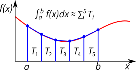
Recall that the area of a trapezoid is the average of its sides times its height. The number of trapezoids shall be read from command line input.

Exercise 14

Approximately calculate π using the statistical method.

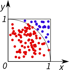
Generate pairs of random numbers (x,y) in the interval [0,1]. If they correspond to a point within the quarter circle, count them as “in”. For large numbers of pairs, the ratio of “in” to the total number of pairs should correspond to the ratio of the area of the quarter circle to the area of the square (as described by the mentioned interval).

To generate (pseudo-)random numbers in Fortran use

real(kind) :: x(dim)
call random_number(x)

Derived Types

When writing your SCF program, you will notice that there are variables that can be grouped or belong to a certain category. To enhance the readability and structure of your code it can be convenient to gather these variables in a so called derived type. A derived type is another data type (like integer or character for example) that can contain built-in types as well as other derived types.

Here is an example of an arbitrary derived type:

type :: arbitrary
  integer     :: num
  real        :: pi
  character   :: string
  logical     :: boolean
end type arbitrary

The derived type contains the four variables num, pi, string and boolean. The syntax to create a variable of type arbitrary and access its members is:

! create variable "arb" of type "arbitrary"
type(arbitrary) :: arb
! access the members of the derived type with %
arb%num = 1
arb%pi = 3.0
arb%string = 'ok'
arb%boolean = .true.

Another advantage of using derived types is that you only need to pass one variable to a procedure instead of all the variables included in the derived type.

Exercise 15

The program below includes a derived type called geometry. So far, it contains the number of atoms and the atom positions. In the rest of the code, two atoms and their positions are set. Then the geometry information is printed by calling the subroutine geometry_info.

1. In order to clearly specify a chemical structure, it is necessary to assign an ordinal number to each atom. Add a one-dimensional allocatable integer variable to the derived type that will contain the ordinal number for each atom. Allocate memory for your new variable and set the initial value to zero using the source expression.

2. Now add a third atom to the geometry and assign atom types and positions to create a sensible carbon dioxide molecule.

3. Add the ordinal number to the printout in the geometry_info subroutine.

derived_types.f90

program derived_types
  implicit none
  intrinsic             :: selected_real_kind
  integer, parameter    :: wp = selected_real_kind(15)

! derived type cleary specifying a chemical structure
type :: geometry
  !> number of atoms
  integer               :: n
  !> xyz coordinates of the atoms in angstrom
  real(wp), allocatable :: xyz(:,:)
end type
  
  type(geometry)        :: geo


! define number of atoms
geo%n = 2

! allocate memory for atoms  and set initial values to zero
allocate(geo%xyz(3, geo%n), source=0.0_wp)

! define atom types and positions
! first atom is oxygen
geo%xyz(1,1) = -1.16_wp
! second atom is carbon

! third atom is oxygen


call geometry_info(geo)


contains

subroutine geometry_info(geo)
  type(geometry)    :: geo
  integer           :: i
  write(*,'(a, i0, a)') 'The input geometry has ', geo%n, ' atoms.'
  write(*,'(a)') 'Writing atom positions:'
  do i=1, geo%n
    write(*,'(3f10.4)') geo%xyz(:,i)
  enddo
end subroutine geometry_info


end program derived_types

Solutions 15

derived_types.f90

program derived_types
  implicit none
  intrinsic             :: selected_real_kind
  integer, parameter    :: wp = selected_real_kind(15)

! derived type cleary specifying a chemical structure
type :: geometry
  !> number of atoms
  integer               :: n
  !> xyz coordinates of the atoms in angstrom
  real(wp), allocatable :: xyz(:,:)
  !> atom type
  integer, allocatable  :: at(:)
end type
  
  type(geometry)        :: geo


! define number of atoms
geo%n = 3

! allocate memory for atoms  and set initial values to zero
allocate(geo%xyz(3, geo%n), source=0.0_wp)
allocate(geo%at(geo%n), source=0)

! define atom types and positions
! first atom is oxygen
geo%at(1) = 8
geo%xyz(1,1) = -1.16_wp
! second atom is carbon
geo%at(2) = 6
! third atom is oxygen
geo%at(3) = 8
! carbondioxide should be linear and symetric
! therefore the x-coordinate of the new oxygen should be 1.16 angstrom
geo%xyz(1,3) =  1.16_wp

call geometry_info(geo)


contains

subroutine geometry_info(geo)
  type(geometry)    :: geo
  integer           :: i
  write(*,'(a, i0, a)') 'The input geometry has ', geo%n, ' atoms.'
  write(*,'(a)') 'Writing atom positions followed by atom type:'
  do i=1, geo%n
    write(*,'(3f10.4,4x,i0)') geo%xyz(:,i), geo%at(i)
  enddo
end subroutine geometry_info


end program derived_types