Exercises#
Electron Correlation#
Multireference Methods#
Exercise 1.1
Electron correlation is very important in dissociation processes to get qualitatively and quantitatively correct results. Calculate the potential energy curves for the dissociation of HF with the single-reference methods RHF, UHF, MP2, CCSD(T) and CASSCF, which is a multi-reference method. Compare the results.
Approach
In order to easily calculate potential energy curves, we use ORCA. Create the following inputs for the given methods and save them in different directories. (e.g.
rhf.inp,uhf.inp, etc.).Input for RHF:
1! RHF def2-TZVP TightSCF
2
3%paras R= 4.0,0.5,35 end
4
5* xyz 0 1
6H 0 0 0
7F 0 0 {R}
8*
Modifications for
UHF:
1! UHF def2-TZVP TightSCF
2
3%scf BrokenSym 1,1 end
MP2:
1! RHF MP2 def2-TZVP TightSCF
CCSD(T):
1! RHF CCSD(T) def2-TZVP TightSCF
CASSCF (2 active electrons in 2 orbitals):
1! RHF def2-TZVP TightSCF Conv
2
3%casscf
4  nel 2
5  norb 2
6  switchstep nr
7end
Calculate the potential energy curve by a CASSCF calculation with 6 electrons (
nel) in 6 active orbitals (norb) as well.Call ORCA with the command
orca <file>.inp > <file>.out
Plot the resulting potential energy curves e.g. using
gnuplot(see section Plotting). To do so, delete the first line in the files<filename>.trj*.datto read them (find out which file is the right one yourself).Calculate the energies for hydrogen and fluorine atoms for all given methods. Which methods will yield the identical energies for the hydrogen atom?
Plot the curves relative to the energies of the individual atoms and discuss your results (particularly the energies at large distances).
Hint
Have a closer look at the UHF dissociation curve. Does it look as you would expect it? Try to explain the “strange” behavior in terms of symmetry breaking.
Hint
If you encounter convergence problems in the CAS(6,6) calculations, try increasing the
maximum number of macro-iterations for CASSCF by adding the following keyword in the
%casscf block:
6 maxiter 1000
Carbenes#
All following calculations will be done with TURBOMOLE if not stated otherwise. Also, if not specified otherwise we will use the RI approximation and C1 symmetry throughout.
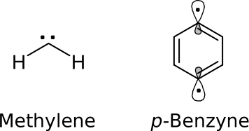
Exercise 1.2
Calculate the singlet-triplet splitting of methylene and p-benzyne with HF, MP2, DFT and CCSD(T).
Approach
Create the file
coordwith starting geometries for Methylene and p-Benzyne.The syntax is:
1$coord
2x y z atom1
3x y z atom2
4...
5...
6$end
You can either create the files by hand or use the program
Avogadrofor this purpose (see section Software for Visualization of Molecules).Avogadrouses Å as unit, but the unit for thecoordfile has to be bohr (atomic units). To convert a *.xyz file into a coord file you can use the commandx2t *.xyz > coord
This also works the other way round:
t2x coord > *.xyz
Methylene: Optimize the geometries of the singlet and the triplet state with the given methods (HF, TPSS, B3LYP, PW6B95, MP2) and the basis set def2-TZVP. The following input is an example of a
controlfile with the correct options for a B3LYP/def2-TZVP calculation of the triplet (= 2 unpaired electrons) state.1$coord file=coord 2$eht charge=0 unpaired=2 3$symmetry c1 4$atoms 5 basis=def2-TZVP 6$dft 7 functional b3-lyp 8$rij 9$energy file=energy 10$grad file=gradient 11$end
To generate the input for the other calculations, please look at the table provided in section Keywords in control. For the MP2 calculations, exchange the$dftwith the proper$ricc2block and don’t forget to specify$denconvsmall enough.Geometry optimizations (DFT, HF) are done with the programjobex:jobex -ri > jobex.out
Note that for MP2 geometry optimizations, you have to add the
-level cc2option. Energies after geometry optimizations can be found in the filejob.last. HF and DFT energies for each SCF-cycle are additionally written in the fileenergy. In the case of CCSD(T) (also defined via the$ricc2block), do not perform a geometry optimization, but do a single-point calculation on the MP2 optimized geometries. Before performing the actual CCSD(T) calculation, you have do run a HF-SCF:ridft > ridft.out ccsdf12 > ccsdf12.out
The energies can then be found in
ccsdf12.out.In order to measure the angles of the optimized structures, you can use
Avogadroor a small TURBOMOLE script calledbend:bend i j k
with atom numbersi,j,k.Note down the HCH-angle and total energies for each method, as well as the singlet-triplet splitting (\(\Delta E_\text{S-T} = E_\text{singlet} - E_\text{triplet}\)). The experimental value for the splitting is 9.0 kcal⋅mol-1. The experimentally found angles are 102.4° for the singlet and 135.5° for the triplet.p-Benzyne: Repeat the same calculations for p-benzyne. The experimental value for the splitting is -4.2 kcal⋅mol-1.
Discuss your findings and compare them to the experiment.
Hint
A HF calculation can be performed by simply omitting the $dft block in the above
input file. For post HF calculations, add the $ricc2 block:
1$ricc2
2  mp2                # or ccsd(t)
3  geoopt model=mp2   # only for MP2 geometry optimizations
Hint
If you encounter convergence problems in the MP2 or CCSD(T) calculations, try to increase the maximum number of SCF cycles (e.g. 100) by adding the following keyword:
1 $scfiterlimit <limit>
Basis Set Convergence#
Formic Acid Dimer#
Exercise 2.1
Investigate the basis set convergence behavior of different methods for the formic acid dimer.
Approach
Create separate directories for the formic acid dimer and monomer and set up geometry optimizations on the TPSS-D3/def2-TZVP level of theory. To do so, create structures using e.g.
Avogadroand convert them tocoordfiles. Prepare the calculations in the same way as in exercise 1.2. You can use a similarcontrolfile and add the$disp3 -bjkeyword for the D3 dispersion correction. DFT geometry optimizations are performed via:jobex -ri > jobex.out
Using the optimized geometries, calculate the dimerization energy (energy difference of one dimer and two monomers) with HF, TPSS-D3 and MP2 employing the cc-pVXZ (X = D, T, Q) basis sets and their augmented counterparts (aug-cc-pVXZ). Refer to the table of input options given in section Keywords in control.
Tabulate your results and plot the total energies versus the cardinal number of the basis set for each method (e.g. with
gnuplot).Discuss your findings with respect to the basis set superposition error (BSSE) and the basis set incompleteness (BSIE).
Which methods can be considered as converged towards the basis set limit when used with a quadruple-ζ basis? Is this expected from theory?
Hint
The calculations with quadruple-ζ basis can be quite time consuming. Exploiting the symmetry by choosing the correct point group in the
$symmetryblock might accelerate the calculations.Remember that you have to perform a HF single-point calculation (using
ridft) before you can start the MP2 calculation withricc2in the same directory.
Thermochemistry#
Reaction Enthalpies of Gas-Phase Reactions#
Exercise 3.1
For small molecules, highly accurate thermochemical results are reachable in quantum chemistry. This means chemical accuracy with an error of less than 1 kcal/mol. Calculate the reaction enthalpies at 298 K for the following, industrially important reactions:
The experimental data are:
Reaction |
\(\Delta H_{r}(298\,\text{K})\) / kcal⋅mol-1 |
|---|---|
Steam reforming |
+49.3 |
Haber-Bosch |
-22.5 |
Approach
Optimize the reactants and products using TPSS-D3/def2-TZVP (see earlier exercises and section Keywords in control, keep in mind the
$disp3 -bjkeyword).In order to get the thermal corrections from energy to enthalpy at 298 K, do a frequency calculation first. Use the program
aoforceto calculate the vibrational frequencies in TURBOMOLE:aoforce > aoforce.out
Then, calculate the thermal enthalpy corrections \(\Delta H_{298}\) with the program
thermo. It needs a.thermorcinput file from your home directory. Create this file by typing:echo "0.0 298.15 1.0" > ~/.thermorc
The first number is an internal threshold, the second the temperature in Kelvin and the third the scaling factor for the vibrational frequencies (1.0 for TPSS). Pipe the output into a separate file, e.g.:
thermo > thermo.out
Repeat the optimization for the molecules involved in the Haber-Bosch process with MP2/def2-TZVP. Calculate the deviation of these differently optimized structures by computing the root mean square deviation of the coordinates:
rmsd <tpss-geometry> <mp2-geometry>
Calculate single-point energies with the hybrid functional B3LYP-D3/def2-TZVP and with MP2/def2-TZVP. Use the TPSS-D3 geometries and thermal corrections to calculate the reaction enthalpies.
Calculate single-point energies with the double hybrid B2PLYP-D3/def2-QZVP and with CCSD(T)/def2-QZVP. Use the TPSS-D3 geometries and thermal corrections to calculate the reaction enthalpies. Keep in mind that you have to run an SCF first with
ridft. Afterwards, usericc2for the double-hybrid andccsdf12for the coupled cluster calculation. The energies can be found in the respective output.Tabulate your results and compare to the experimental values. Which method would you expect to show the smallest deviation to the experiment? Do your findings match your expectation? Disscuss your outcome.
Heat of Formation of C60 (optional)#
Exercise 3.2
Calculate the heat of formation \(\Delta H_f^0\) of the C60 molecule by using different methods.
Approach
Optimize the geometry of C60 on the TPSS-D3/def2-SVP level in Ih symmetry. In order to do so you can build a
coordfile on your own or search for a proper input on the internet. The symmetry can be defined with the$symmetry ihkeyword incontrol.Calculate the energy of C60 on TPSS/def2-SVP level without D3 corrections, use the TPSS-D3/def2-SVP optimized geometry.
Calculate the frequencies of C60 and the thermal corrections the same way as in exercise 3.1.
Now, calculate the energy of a single carbon atom on the TPSS/def2-SVP level of theory and the thermal corrections to \(\Delta H_{298.15}\) (use C1 symmetry).
Calculate \(\Delta H_f^0\) of C60 and compare to experimental results (599 / 635 kcal/mol). You will need the experimental \(\Delta H_f^0\) of a carbon atom: 170.89 kcal/mol.
Calculate single-point energies (without dispersion correction) for carbon and C60 with TPSS and HF employing the def2-TZVP and the def2-QZVP basis sets. Use the results to calculate the heat of formation. (Use the TPSS-D3/def2-SVP geometries and corrections to \(\Delta H_{298.15}\) for this purpose.)
Calculate the D3 dispersion correction to the TPSS/def2-QZVP energy and calculate \(\Delta H_f^0\) again. Use the standalone program
dftd3:dftd3 coord -func tpss -bj
Discuss your results.
Kinetics#
Kinetic Isotope Effect#
Exercise 4.1
Calculate the kinetic isotope effect for the reaction CH4 + HO⋅ → ⋅CH3 + H2O. From transition state theory, it is known that
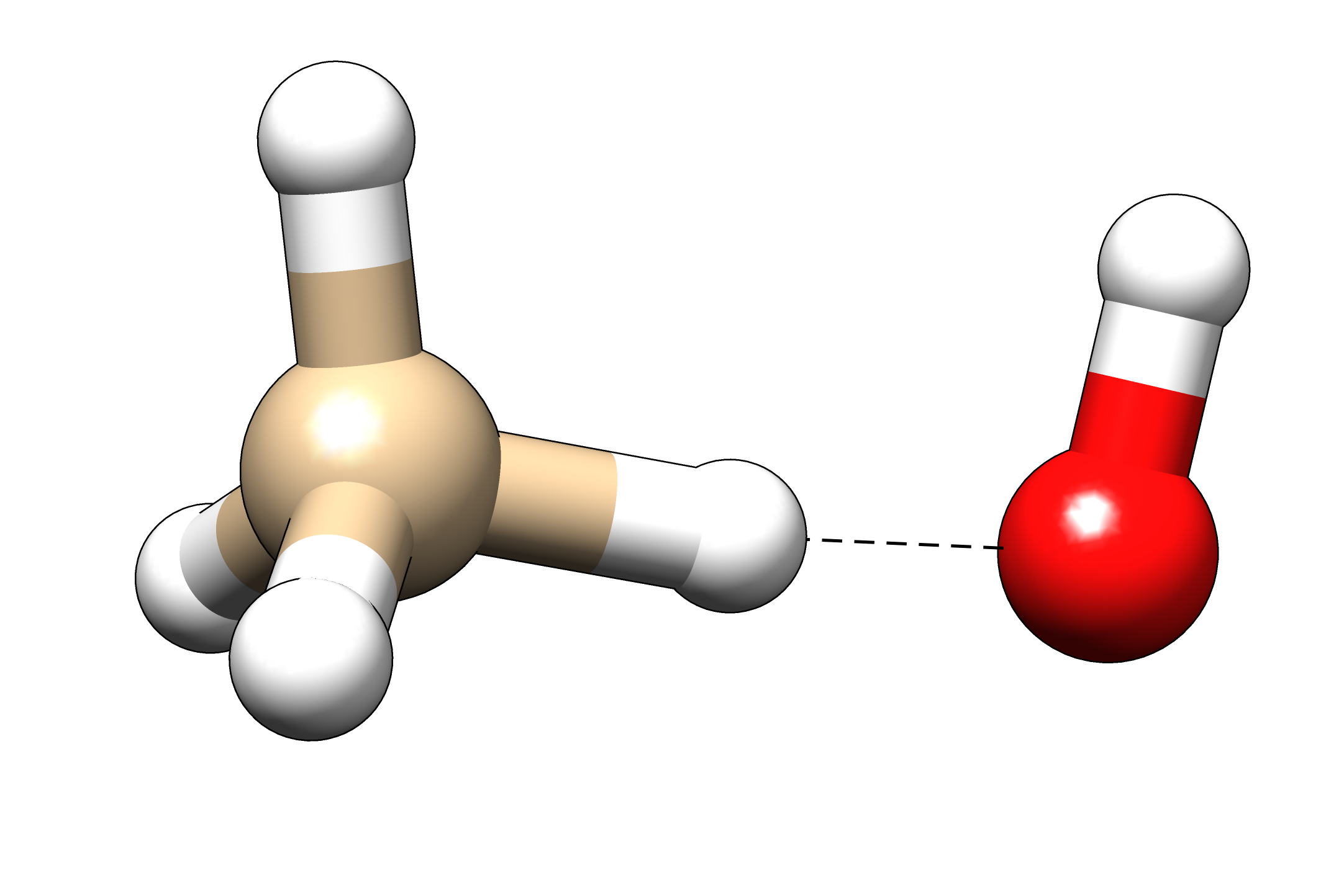
Geometry of the transition state.#
Approach
Calculate the geometry of the transition state for the hydrogen transfer. In order to do this, create a
coordfile with a starting geometry that is similar to the one in the picture, with \(R_{C-H} \approx\) 1.2 Å and \(R_{O-H} \approx\) 1.3 Å.In order to find the transition state, use the following steps:
Prepare a
controlfile. Use the B3LYP-D3/def2-TZVP level of theory. Look at section Keywords in control if you are unsure. You might need to increase the$scfiterlimitin this exercise.Consecutively, calculate energy, gradient and hessian:
ridft > ridft.out
rdgrad > rdgrad.out
aoforce > aoforce.out
Verify that there is at least one, relatively large imaginary frequency in the output of
aoforce(it also appears in thevibspectrumfile). Then, add the following block to thecontrolfile.1$statpt 2 itrvec 1
(in general the frequency mode describing the motion of the reaction)
Start the transition state search:
jobex -ri -trans > jobex.out
When the search is successful (a
GEO_OPT_CONVERGEDfile has been created in the directory), calculate the vibrational frequencies of the transition state (aoforce) and verify that there is only one imaginary frequency. You can have a look at that corresponding normal mode by calling:tm2molden
Choose your desired options in the short interactive experience. You do not need to pick a name for the input file or to save the MO data, the latter will make the file rather large (but obviously save the frequency data). You can open the resulting file (default:
molden.input) withgmolden. The normal modes can be visualized by clicking on “Norm. Mode” on the right side of the menu.Call the program
thermoand note down the thermal corrections to the enthalpy.Repeat the transition state search with CD4 and OH. Therefore, take the initial
controlfile and add an additional non-default atom weight definition to the 4 affected hydrogen atoms in the$atomsblock. You need to look in thecoordfile and identify the indices of thehatoms you want to change to deuterium. Say these hydrogen atoms are atoms 2, 3, 4 and 5, then change the$atomsblock to:1$atoms 2 basis=def2-TZVP 3h 2,3,4,5 4 mass=2.014
With this input, repeat all aforementioned steps.
Calculate the energies and thermal corrections for CH4, CD4 and OH.
Finally, calculate \(k_\text{H}/k_\text{D}\).
Solvation#
SN2-Reaction#
Exercise 5.1
Calculate the potential energy curve for the SN2-reaction of chloromethane with a flouride anion in the gas-phase and in methanol (ε = 32) between \(r(\text{C}-\text{F})\) = 2.25 and 8.00 bohr with ε being the dielectric constant of the solvent.
Approach
Create structures and calculate the energies of the reactants (one calculation for each reactant) in the gas-phase and at ε = 32 (methanol). Use the hybrid functional PW6B95 with a def2-TZVP basis and D3 dispersion correction. Keep in mind that you also have to specify the charge and the solvent model in the
controlfile, e.g.:1$eht charge=-1 unpaired=0 2$cosmo 3 epsilon=32.0
If you run into problems running the constrained optimizations, try adding the following to your control file:
1$optimize
2 internal off
3 cartesian on
To create the potential energy curves, use the shell script below. The script loops over all distances. For each distance it creates a new directory, performs the constrained geometry optimization and writes the electronic energy (not necessarily your final reaction energy) into a file called
results.dat. Create a new directory and copy and paste the script to a file namedrun-scan.sh.1#!/usr/bin/env bash 2 3# Choose directory here 4calc_dir=scan_vac 5 6cd $calc_dir 7if [ -f ./results.dat ] 8then 9 rm results.dat 10fi 11 12read -r -d 'END' template <<-EOF 13\$coord 14 0.00000000 0.00000000 0.00000000 c f 15 0.00000000 0.00000000 -3.36989165 cl 16 0.00000000 0.00000000 DIST f f 17 -1.00404366 1.73905464 -0.62462166 h 18 -1.00404366 -1.73905464 -0.62462166 h 19 2.00808733 0.00000000 -0.62462166 h 20\$end 21END 22EOF 23 24for dist in $(seq 2.25 0.25 8.00 | sed s/,/./) 25do 26 27 # Check for existence of folder 28 if [ -d $dist ] 29 then 30 rm -r $dist 31 fi 32 mkdir $dist 33 cp control $dist 34 pushd $dist 35 echo "$template" | sed "s/DIST/$dist/" > coord 36 37 jobex -ri -c 50 38 39 # Get final energy 40 e=$(sdg energy | tail -1 | gawk '{printf $2}') 41 42 # Write energy to a file 43 echo $dist $e >> ../results.dat 44 popd 45 46done
A template for the
coordfile is given directly inline in the script, we will repeat it here to explain a few details. Thefafter the atom specification tells TURBOMOLE to keep the coordinates fixed for that atom.DISTist a placeholder which will be substituted by the C–F distance.13$coord 14 0.00000000 0.00000000 0.00000000 c f 15 0.00000000 0.00000000 -3.36989165 cl 16 0.00000000 0.00000000 DIST f f 17 -1.00404366 1.73905464 -0.62462166 h 18 -1.00404366 -1.73905464 -0.62462166 h 19 2.00808733 0.00000000 -0.62462166 h 20$end
In order to use the script, you have to make it executable by typing:
chmod +x run-scan.sh
Create subdirectories (e.g.
scan_vacandscan_cosmo) for each potential energy curve and place a propercontrolfile in each of these subdirectories. You will have to adapt the script to your directory names (name in line 4). Theresults.datfile will be written to the respective subdirectory. Execute the script by typing:./run-scan.sh
Plot the two curves together (normalize the curves reasonably) and discuss the results. Estimate the activation barrier for both cases.
Hint
If the execution of such a script takes some longer time, consider calling it with:
nohup ./run-scan.sh &
Then, you can log out of your shell without killing the calculation.
Activation Energies#
Rearrangement and Dimerization Reactions#
Exercise 6.1
Estimate the activation energy for the Claisen rearrangement of allyl-vinyl ether and the dimerization of cyclopentadiene to endo-dicyclopentadiene (Diels-Alder).
Approach
Construct the geometry of reactant(s) and product for each reaction (e.g. using
Avogadro). Ensure that the sequence of atoms is the same in every pair of reactant and product structure.Hint
Preparing good input structures for transition state searches is absolutely essential, often you can easily create a product structure from your reactant. Furthermore, this generally eases the sorting of the atoms.
Optimize the geometries using GFN2-xTB. GFN2-xTB is a semi-empirical tight-binding based method that employs a minimal valence basis set and is very efficient for calculating Geometries, vibrational Frequencies and Noncovalent interactions. For running the geometry optimization, call
xtb start.xyz --opt > opt.out
The optimized geometry is written to the file
xtbopt.xyz.Verify that the sequence of atoms is still the same in every pair of reactant and product structure.
Perform a reaction path search with the double-ended Growing String Method (GSM) at the GFN2-xTB level:
Create a directory for each reaction.
Have your optimized reactant and product structure sorted and available in xyz format (e.g. starting structure
start.xyz, ending structureend.xyz).Create a directory
scratchand store the starting and ending structures in the fileinitial0000.xyz:cat start.xyz end.xyz >> scratch/initial0000.xyz
Place a file named
ogradin the respective directory with the following content:1#!/bin/bash 2ofile=orcain$1.in 3ofileout=orcain$1.out 4molfile=structure$1 5ncpu=$2 6basename="${ofile%.*}" 7########## XTB/TM settings: ################# 8cd scratch 9wc -l < $molfile > $ofile.xyz 10echo "Dummy for XTB/TM calculation" >> $ofile.xyz 11cat $molfile >> $ofile.xyz 12 13xtb $ofile.xyz -grad > $ofile.xtbout 14 15tm2orca.py $basename 16rm xtbrestart 17cd ..
The
ogradfile has to be made executable:chmod u+x ograd
Place a file named
inpfileqin the respective directory with the following content:1# FSM/GSM/SSM inpfileq 2 3------------- QCHEM Scratch Info ------------------------ 4$QCSCRATCH/ # path for scratch dir. end with "/" 5GSM_go1q # name of run 6--------------------------------------------------------- 7 8------------ String Info -------------------------------- 9SM_TYPE GSM # SSM, FSM or GSM 10RESTART 0 # read restart.xyz 11MAX_OPT_ITERS 160 # maximum iterations 12STEP_OPT_ITERS 30 # for FSM/SSM 13CONV_TOL 0.0005 # perp grad 14ADD_NODE_TOL 0.1 # for GSM 15SCALING 1.0 # for opt steps 16SSM_DQMAX 0.8 # add step size 17GROWTH_DIRECTION 0 # normal/react/prod: 0/1/2 18INT_THRESH 2.0 # intermediate detection 19MIN_SPACING 5.0 # node spacing SSM 20BOND_FRAGMENTS 1 # make IC's for fragments 21INITIAL_OPT 0 # opt steps first node 22FINAL_OPT 150 # opt steps last SSM node 23PRODUCT_LIMIT 100.0 # kcal/mol 24TS_FINAL_TYPE 0 # 0=no bond breaking, 1=breaking of bond 25NNODES 15 # including endpoints 26---------------------------------------------------------
For the Claisen rearrangement, you can change the
TS_FINAL_TYPEoption from 0 to 1 to force GSM to break a bond upon the transition state search. The number of nodes (keywordNNODES) can be increased for a more refined search, which (of course) leads to longer computing time. In most cases, 15 nodes should be sufficient to find a good guess for the transition state.
Start the transition state search by typing:
gsm.orca
After the calculation, you can find the reaction path in the file
stringfile.xyz0000, and the transition state inscratch/tsq0000.xyz.
Prepare relative energy diagrams for both reactions (relative energy vs. reaction coordinate), depict the molecular structures of both transition states and highlight the most important bond distances.
Calculate the activation energy for each reaction.
Perform single-point calculations on the starting structure and transtion state structure with PW6B95-D3/def2-TZVP using TURBOMOLE. Compare the DFT activation energy with the GFN2-xTB energy and discuss the differences.
How would you proceed further to gain more reliable numbers?
How feasible is this approach? Where do you see its limits in applicability and usefulness?
Noncovalent Interactions#
Noble Gas ⋅ ⋅ ⋅ Methane#
Exercise 7.1
Calculate potential energy curves of the “weak” interactions between the noble gases Ar or Kr and methane.
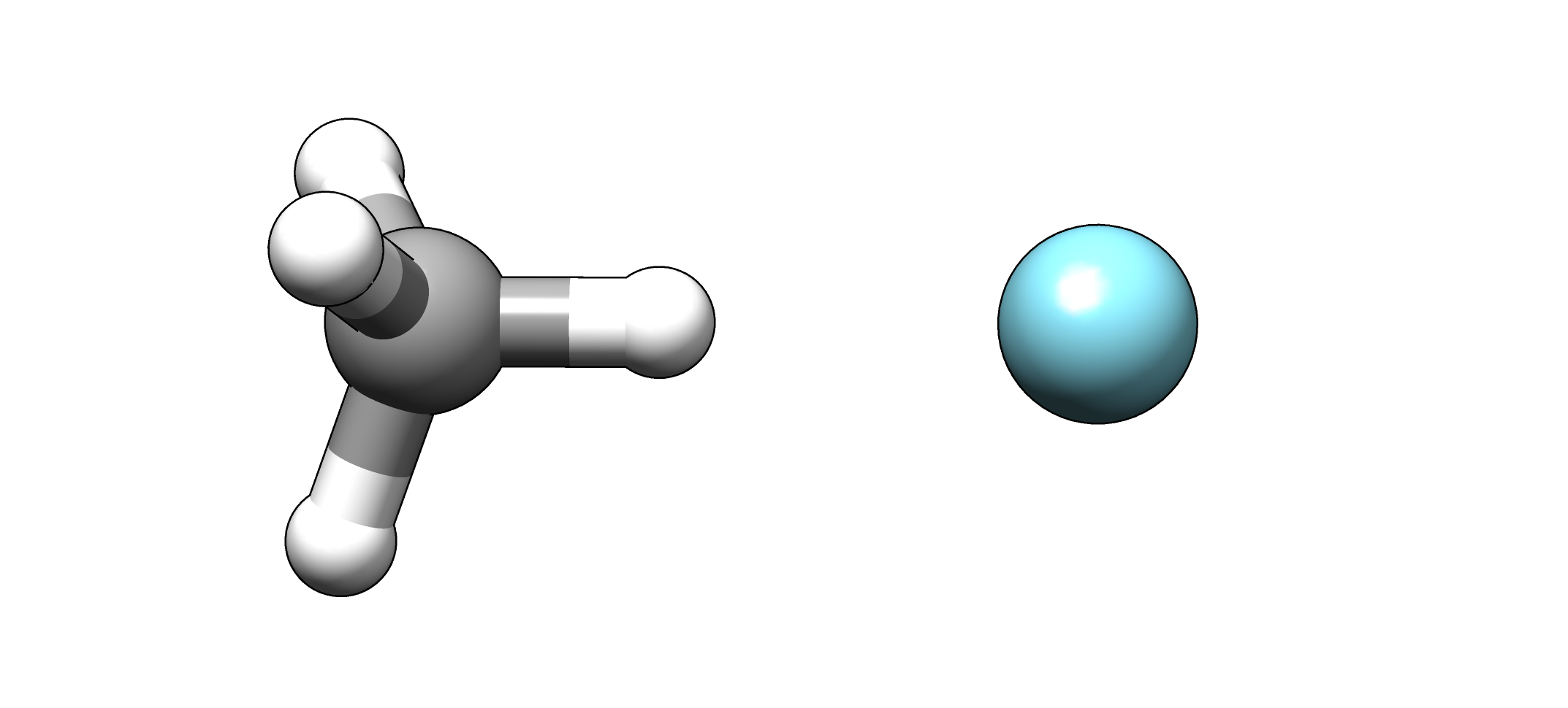
Geometry of the CH4 ⋅ ⋅ ⋅ Ar complex.#
Approach
- Calculate the potential energy curve at the BLYP-D3/def2-QZVP level for Ar ⋅ ⋅ ⋅ HCH3 by performing a geometry optimization with a fixed Ar and H atom. Do this for \(R_\text{(Ar-H)}\) = 4.5 - 15.0 bohr with a stepsize of 0.25 bohr.Use the
run-scan.shscript from exercise 5.1 and adopt it to this task. Substitute the template molecular geometry by the following one:13$coord 14 0.00000000000000 0.00000000000000 DIST ar f 15 0.00000000000000 0.00000000000000 0.00000000000000 h f 16 0.00000000000000 0.00000000000000 -2.06945348098289 c 17 0.97576020317533 1.69006623336522 -2.75977586481614 h 18 0.97576020317533 -1.69006623336522 -2.75977586481614 h 19 -1.95152040635065 0.00000000000000 -2.75977586481614 h 20$end
You also have to modify the directory names and the distances. Prepare a
controlfile for the BLYP-D3/def2-QZVP calculations including the$disp3 -bjand$symmetry c1keywords. Repeat the calculations for BLYP/def2-QZVP and MP2/def2-QZVP. For BLYP, just omit the
$disp3block. For MP2, clear the$dftand$disp3blocks and insert proper settings under$ricc2and$denconv. In the latter case, don’t forget to change thejobexcommand in the script to:37 jobex -ri -level cc2 -c 50
To get the final MP2 energy for each distance, also change the
sdgcommand to:40 e=$(grep "Total Energy" job.last | gawk '{print $4}')
Repeat the calculations for Kr ⋅ ⋅ ⋅ HCH3 (substitute
arbykrin the template) with BLYP-D3/def2-QZVP, BLYP/def2-QZVP and MP2/def2-QZVP.Plot the curves (normalize to the dissociation limit) and discuss your findings.
Spectroscopy#
IR-Spectrum of 1,4-Benzoquinone#
Exercise 8.1
Calculate the IR-spectrum of 1,4-benzoquinone using DFT and HF, and compare the results to the experimental spectrum given below.
Approach
Create a
coordfile for 1,4-benzoquinone.Optimize the geometry with TURBOMOLE on the HF-D3/def2-SVP level of theory.
Calculate the normal modes with
aoforce.Call
tm2moldenand check the normal modes withgmoldenthe same way as in exercise 4.1.Assign each dipole-allowed normal mode to an experimental one and calculate the scaling factor \(f_\text{scal}=\nu_\text{exp}/\nu_\text{calc}\).
Repeat everything with TPSS-D3/def2-SVP and discuss your findings.
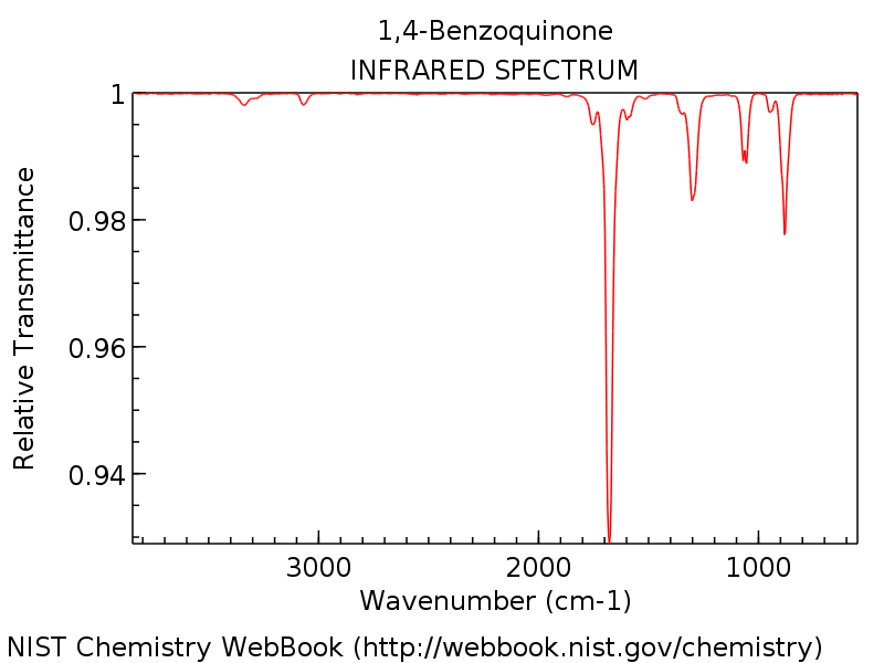
IR spectrum of 1,4-benzoquinone in KBr.#
Hint
If you obtain imaginary frequencies, try to start the geometry optimization from a slightly distorted structure. Check if the imaginary frequencies vanish.
The Color of Indigo#
Exercise 8.2
Calculate the color of indigo with three different methods: time-dependent Hartree-Fock (TD-HF) and time-dependent DFT (TD-DFT) with two different functionals (PBE and PBE0).
Approach
In this exercise, please use TURBOMOLE’s interactive input generator
defineto create thecontrolfile. To do so, create the geometry of an indigo molecule (figure below) and place thecoordfile in its own directory.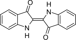
Structure of indigo.#
To start the input generator, navigate to the directory containing the
coordfile, type the following command and answer all questions that appear.define
Prepare an input on the TPSS-D3/def2-SVP level and optimize the geometry. In the define dialogue, you can skip the first two questions, then choose the input geometry file via:
a coordIn this menu, you will find a header telling you the number of atoms of your molecule and its symmetry point group (Schoenflies symbol). If this is not yet correct (the molecule does not have C1 symmetry), typedesy 1d-3or some larger value to loosen the symmetry determination threshold until the correct point group is recognized. If the symmetry is still not recognized correctly, you can set the point group manually with thesycommand. In this case make sure TURBOMOLE does not add atoms to yourcoordfile.Leave the molecular geometry menu and then do not choose internal coordinates. In the atomic attribute definition menu, you can choose the same basis for all atoms by typing e.g.:b all def2-SVP
Afterwards, choose an extended Hückel guess for the MOs with default parameters (don’t worry about a small HOMO/LUMO gap). In the last general menu, go to the
dftsubmenu and type e.g.:on func tpssDon’t forget to also choose the
bjoption in thedspsubmenu for the D3 disperion correction (activating the RI approximation in therisubmenu is also recommended). When you are finished, you will find acontrolfile in your directory containing all keywords you already know and more. If everything is correct, you are now ready to run the geometry optimization.Hint
Try to navigate through the
definedialogue a few times and explore it by yourself to get familiar with it. If you still can’t figure out a certain aspect, feel free to ask your lab assistant.Prepare a HF-D3/def2-SVP single-point calculation in the same way by using
define, but do not turn on thedftoption. Do not use the RI approximation here and run:dscf > dscf.out
In order to do the subsequent TD-HF (or a TD-DFT) calculation, add the following two blocks so the
controlfile:1$scfinstab rpas 2$soes 3 bu 1
Then, run:
escf > escf.out
For the TD-DFT calculations repeat the above procedure with PBE-D3/def2-SVP and PBE0-D3/def2-SVP (now with RI approximation). Use proper settings during the
definedialogue as well as incontroland run:ridft > ridft.out escf > escf.out
Discuss the excitation energies for all three methods; which method would predict (at least approximately) the correct color for indigo? How do you explain the errors?
NMR Parameters#
The computation of NMR parameters can be done with the ORCA program package. A simple input for the calculation of the NMR chemical shielding of CH3NH2 with the PBE functional and a pcSseg-2 basis set is presented below. The pcSseg-n basis sets are special segmented contracted basis sets otimized for the calculation of NMR shieldings. (For more information see: Jensen, F., J. Chem. Theory Comput. 2015, 11, 132 - 138.)
1!PBE RI pcSseg-2 def2/J NMR
2
3*xyzfile 0 1 input.xyz
At the end of the ORCA output, a summary of the calculated NMR absolute chemical shieldings can be found.
Exemplary output for CH3NH2:
 1--------------------------
 2CHEMICAL SHIELDING SUMMARY (ppm)
 3--------------------------
 4
 5
 6  Nucleus  Element    Isotropic     Anisotropy
 7  -------  -------  ------------   ------------
 8      0       C          152.992         46.821
 9      1       H           29.025          8.165
10      2       H           28.567         10.286
11      3       N          242.339         43.497
12      4       H           29.033          8.176
13      5       H           31.095         13.580
14      6       H           31.120         13.593
Exercise 8.3
Calculate the 13C-NMR chemical shifts δ for a number of organic compounds and compare the results to experimental data. In addition, investigate the correlation of the π-electron density with δ.

Lewis structures of four organic compounds A – D with their experimentally obtained chemical shift as well as four aromatic compounds Ar-1 - Ar-4.#
Approach
Optimize the geometries of the compounds A – D and the reference molecule Si(CH3)4 (TMS) on the PBEh-3c level of theory (how to use PBEh-3c is explained in the ORCA manual).
Calculate the 13C-NMR chemical shieldings and shifts δ for compounds A – D with TMS as reference at PBE/pcSseg-2 level of theory (use this level in all the following calculations if not stated otherwise). Given the isotropic NMR shielding constants \(\sigma\) of the compound (\(\text{c}\)) and the reference (\(\text{ref.}\)), the chemical shift \(\delta _\text{c,ref.}\) is defined as
\[\delta _\text{c,ref.} = \sigma _\text{ref.} - \sigma _c .\]Hint
Computational time can be saved by calculating the shieldings only for carbon atoms instead of all atoms. How to do so is described in the ORCA manual.
Compare your results with the experimental values and calculate the mean deviation (MD) and the mean absolute deviation (MAD). How meaningful are these statistical measures for the given sample size?
\[\text{MD} = \frac{1}{N} \sum_{i=1}^N (\delta _\text{calc.} - \delta _\text{exp.}) \hspace{1.5cm} \text{MAD} = \frac{1}{N} \sum_{i=1}^N (|\delta _\text{calc.} - \delta _\text{exp.}|)\]Repeat the calculations for the four aromatic compounds Ar-1 – Ar-4 and plot the calculated chemical shift against the formal π-electron density (\(\rho_\pi = n_{el^\pi}/n_{at^\pi}\)). Discuss your results.
The experimental 17O- and 13C-NMR chemical shifts of the carbonyl function in acetone are shifted by -75.5 and 18.9 ppm, respectively, if an acetone molecule is transferred from the gas phase to aqueous solution. Try to reproduce these values by considering solvation effects by the implicit solvent model CPCM. You can switch on the implicit solvent by adding the
CPCM(<solvent>)keyword (example:CPCM(toluene)) to your ORCA input. For carbon, the reference is TMS, for oxygen it is water.Try to estimate which effect is larger – the inclusion of an implicit solvation in the NMR calculation or the inclusion of the implicit solvent in the geometry optimization.
Hint
There are two options (gas/solution) for each calculation, the geometry optimization and the shielding calculation. Compare all possibilities.
Calculate the 1H-NMR chemical shifts for H and I in the gas-phase at the PBE/pcSseg-2//PBEh-3c level of theory (again use TMS as the reference). Discuss your observations regarding the chemical shift of the methine proton in both compounds. Give a short explanation of your findings.
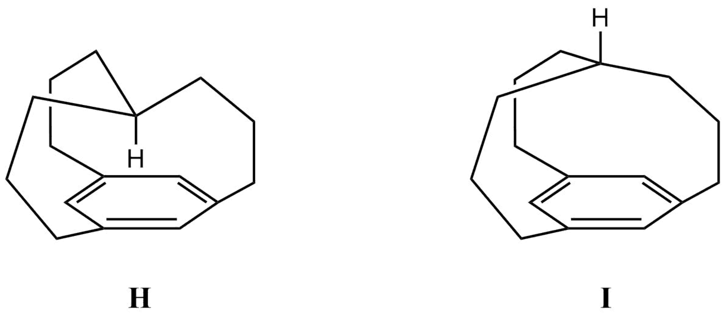
Lewis structures of in- (H) and out- (I) [34,10][7]Metacyclophane.#
Hint
The NMR chemical shielding calculations for H and I may be time consuming, consider to run them over night.